Compute similarity between authors
We can compute the similarities between authors by grouping their documents and comparing them with all other authors. In this example, we group Twitter posts by handle names and compute similarities between the users.
require(quanteda)
require(quanteda.textstats)
require(readtext)
Import Tweets from JSON (.json) file. twitter.json is located in data directory of this tutorial package.
dat_twitter <- readtext("../data/twitter.json", source = "twitter")
Construct a corpus of Tweets.
corp_tweets <- corpus(dat_twitter)
Construct a document-feature matrix, and remove tags, links, and English stopwords.
dfmat_tweets <- corp_tweets %>%
    tokens(remove_punct = TRUE, remove_url = TRUE, remove_symbols = TRUE) %>%
    dfm() %>%
    dfm_remove(pattern = c("*.tt", "*.uk", "*.com", "rt", "#*", "@*")) %>%
    dfm_remove(pattern = stopwords("en"))
ndoc(dfmat_tweets)
## [1] 7504
topfeatures(dfmat_tweets)
##          vote conservatives        labour         today         share
##          1886           959           773           676           649
##       britain          find        fairer      tomorrow        voting
##           639           615           571           570           570
Group documents by Twitter handle names (screen_name).
dfmat_users <- dfm_group(dfmat_tweets, groups = screen_name)
ndoc(dfmat_users)
## [1] 5061
Remove rare (less than 10 times) and short (one character) features, and keep only users with more than 50 tokens in total.
dfmat_users <- dfmat_users %>%
    dfm_select(min_nchar = 2) %>%
    dfm_trim(min_termfreq = 10)
dfmat_users <- dfmat_users[ntoken(dfmat_users) > 50,]
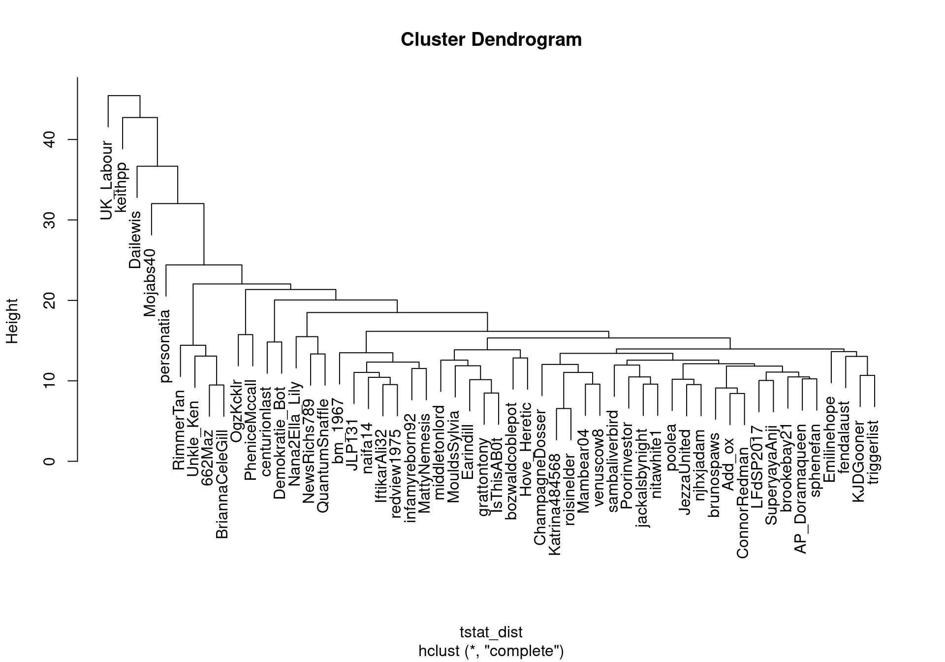
Calculate user-user similarity using textstat_dist().
tstat_dist <- as.dist(textstat_dist(dfmat_users))
user_clust <- hclust(tstat_dist)
plot(user_clust)
