Newsmap
Newsmap is a semi-supervised model for geographical document classification. While (full) supervised models are trained on manually classified data, this semi-supervised model learns from “seed words” in dictionaries.
Install the newsmap package from CRAN.
install.packages("newsmap")
require(quanteda)
require(quanteda.corpora)
require(newsmap)
require(maps)
require(ggplot2)
Download a corpus with news articles using quanteda.corpora‘s download() function.
corp_news <- download(url = "https://www.dropbox.com/s/r8zhsu8zvjzhnml/data_corpus_yahoonews.rds?dl=1")
corp_news contains 10,000 news summaries downloaded from Yahoo News in 2014.
ndoc(corp_news)
## [1] 10000
range(corp_news$date)
## [1] "2014-01-01" "2014-12-31"
Proper nouns are the most useful features of documents for geographical classification. However, not all capitalized words are proper nouns, so we define custom stopwords.
month <- c("January", "February", "March", "April", "May", "June",
           "July", "August", "September", "October", "November", "December")
day <- c("Sunday", "Monday", "Tuesday", "Wednesday", "Thursday", "Friday", "Saturday")
agency <- c("AP", "AFP", "Reuters")
toks_news <- tokens(corp_news, remove_punct = TRUE) %>%
             tokens_remove(pattern = c(stopwords("en"), month, day, agency),
                           valuetype = "fixed", padding = TRUE)
newsmap contains seed geographical dictionaries in English, German, Spanish, Japanese and Russian languages. data_dictionary_newsmap_en is the seed dictionary for English texts.
toks_label <- tokens_lookup(toks_news, dictionary = data_dictionary_newsmap_en,
                            levels = 3) # level 3 is countries
dfmat_label <- dfm(toks_label, tolower = FALSE)

dfmat_feat <- dfm(toks_news, tolower = FALSE)
dfmat_feat_select <- dfm_select(dfmat_feat, pattern = "^[A-Z][A-Za-z0-9]+",
                                valuetype = "regex", case_insensitive = FALSE) %>%
                     dfm_trim(min_termfreq = 10)

tmod_nm <- textmodel_newsmap(dfmat_feat_select, y = dfmat_label)
The seed dictionary contains only names of countries and capital cities, but the model additionally extracts features associated to the countries. These country codes are defined in ISO 3166-1.
coef(tmod_nm, n = 15)[c("US", "GB", "FR", "BR", "JP")]
## as(<matrix>, "dgTMatrix") is deprecated since Matrix 1.5-0; do as(as(as(., "dMatrix"), "generalMatrix"), "TsparseMatrix") instead
## $US
## WASHINGTON         US   American Washington       YORK     States  Americans
##   7.154239   7.036785   6.829831   6.605774   6.369994   6.054570   5.359837
##       York Brunnstrom      Kirby   Platinum      Anglo    Stewart   Keystone
##   4.993287   3.781652   3.701609   3.614598   3.568078   3.162613   3.088505
##    Admiral
##   3.008462
##
## $GB
##   British    LONDON    London   Britain Britain's        UK      UKIP   Kingdom
##  7.877081  7.846983  7.562997  7.264183  6.670409  5.487239  4.905318  4.774289
##     Tesco     Hamza Cameron's   Osborne   Salmond     Clegg   Cameron
##  4.445785  4.358774  3.857999  3.752638  3.695480  3.665627  3.595009
##
## $FR
##        French        France         PARIS         Paris      Hollande
##      8.183063      8.088991      7.541210      7.303251      6.532546
##    Hollande's        Fabius         Valls      Francois Saint-Germain
##      5.401143      5.295783      5.295783      5.277091      4.970361
##        Froome            Le      France's       Renault           Pen
##      4.803306      3.755338      3.734547      3.704694      3.504023
##
## $BR
##    Brazil       SAO     PAULO       RIO   JANEIRO Brazilian       Rio        DE
##  8.174995  7.261448  7.247654  7.048526  7.048526  6.996340  6.922232  6.355378
##   Janeiro       Sao     Paulo      BELO HORIZONTE  BRASILIA     Dilma
##  6.303193  5.966720  5.966720  5.915427  5.915427  5.804201  5.306363
##
## $JP
##        Japan     Japanese        TOKYO          Abe        Tokyo       Shinzo
##     8.166952     7.896661     7.764115     7.063062     6.962979     6.791129
##        Abe's      Tokyo's    Fukushima      Japan's       Nikkei       Toyota
##     5.810299     5.317823     5.171219     4.390779     3.836218     3.479543
##    Pyongyang Asia-Pacific        Honda
##     3.182292     3.156316     3.143071
Names of people, organizations and places are often multi-word expressions. To distinguish between “New York” and “York”, for example, it is useful to compound tokens using tokens_compound() as explained in Advanced Operations.
You can predict the most strongly associated countries using predict() and count the frequency using table().
pred_nm <- predict(tmod_nm)
head(pred_nm, 20)
##  text1  text2  text3  text4  text5  text6  text7  text8  text9 text10 text11
##     KP     SY     IQ     RU     TH     CN     UA     SY     GB     US     SY
## text12 text13 text14 text15 text16 text17 text18 text19 text20
##     US     UA     SY     LK     ES     AU     CR     ID     BH
## 204 Levels: BI DJ ER ET KE MG MU MW MZ RE RW SO TZ UG ZM ZW AO CD CF CG ... WS
Factor levels are set to obtain zero counts for countries that did not appear in the corpus.
count <- sort(table(factor(pred_nm, levels = colnames(dfmat_label))), decreasing = TRUE)
head(count, 20)
##
##  GB  US  RU  UA  AU  CN  CA  FR  IQ  BR  SY  DE  ZA  NZ  JP  IL  IN  ES  EG  PS
## 621 578 516 440 367 362 319 311 295 278 262 250 236 228 198 197 187 182 157 155
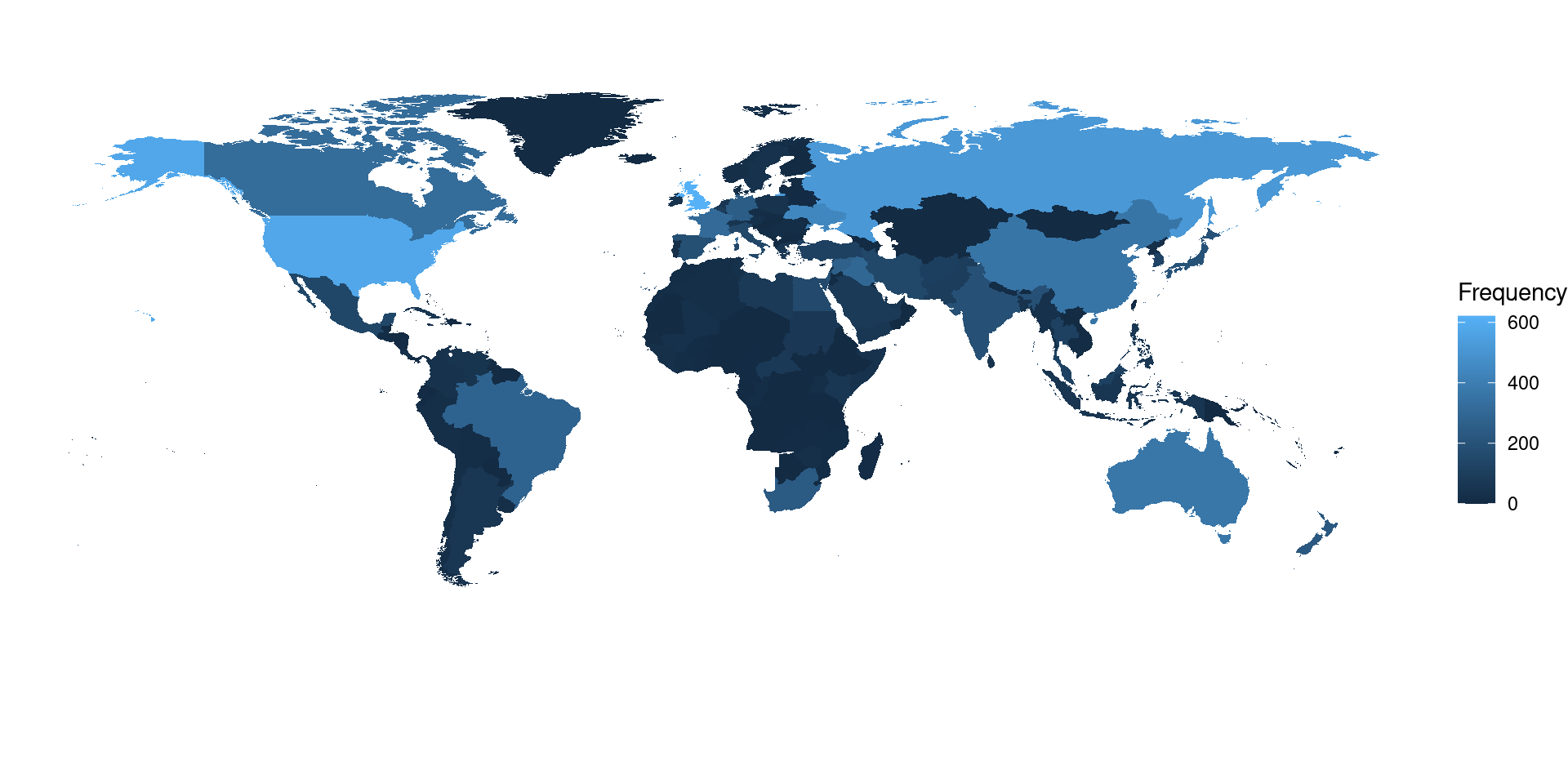
You can visualise the distribution of global news attention using geom_map().
dat_country <- as.data.frame(count, stringsAsFactors = FALSE)
colnames(dat_country) <- c("id", "frequency")

world_map <- map_data(map = "world")
world_map$region <- iso.alpha(world_map$region) # convert country name to ISO code

ggplot(dat_country, aes(map_id = id)) +
      geom_map(aes(fill = frequency), map = world_map) +
      expand_limits(x = world_map$long, y = world_map$lat) +
      scale_fill_continuous(name = "Frequency") +
      theme_void() +
      coord_fixed()
- Watanabe, Kohei. 2018. “Newsmap: A Semi-supervised Approach to Geographical News Classification". Digital Journalism 6(3): 294-309.