Latent Semantic Scaling
Latent Semantic Scaling (LSS) is a flexible and cost-efficient semi-supervised document scaling technique. The technique relies on word embeddings and users only need to provide a small set of “seed words” to locate documents on a specific dimension.
Install the LSX package from CRAN.
install.packages("LSX")
require(quanteda)
require(quanteda.corpora)
require(LSX)
Download a corpus with news articles using quanteda.corpora‘s download() function.
corp_news <- download("data_corpus_guardian")
We must segment news articles into sentences in the corpus to accurately estimate semantic proximity between words. We can also use the Marimo stopwords list (source = "marimo") to remove words commonly used in news reports.
# tokenize text corpus and remove various features
corp_sent <- corpus_reshape(corp_news, to =  "sentences")
toks_sent <- corp_sent %>%
    tokens(remove_punct = TRUE, remove_symbols = TRUE,
           remove_numbers = TRUE, remove_url = TRUE) %>%
    tokens_remove(stopwords("en", source = "marimo")) %>%
    tokens_remove(c("*-time", "*-timeUpdated", "GMT", "BST", "*.com"))

# create a document feature matrix from the tokens object
dfmat_sent <- toks_sent %>%
    dfm() %>%
    dfm_remove(pattern = "") %>%
    dfm_trim(min_termfreq = 5)
topfeatures(dfmat_sent, 20)
##     people        new       also         us        can government       last
##      11168       8024       7901       7090       6972       6821       6335
##        now      years       time      first       just         uk     police
##       5883       5839       5694       5380       5369       4874       4621
##       like      party        get       make       made   minister
##       4582       3890       3852       3844       3752       3680
We will use generic sentiment seed words to perform sentiment analysis.
seed <- as.seedwords(data_dictionary_sentiment)
print(seed)
##        good        nice   excellent    positive   fortunate     correct
##           1           1           1           1           1           1
##    superior         bad       nasty        poor    negative unfortunate
##           1          -1          -1          -1          -1          -1
##       wrong    inferior
##          -1          -1
With the seed words, LSS computes polarity of words frequent in the context of economy. We can identify context words by char_context(pattern = "econom*") before fitting the model.
# identify context words
eco <- char_context(toks_sent, pattern = "econom*", p = 0.05)

# run LSS model
tmod_lss <- textmodel_lss(dfmat_sent, seeds = seed,
                          terms = eco, k = 300, cache = TRUE)
## Reading cache file: lss_cache/svds_402bda98dac8a560.RDS
head(coef(tmod_lss), 20) # most positive words
##        good      status    positive opportunity     success      energy
##  0.12822551  0.09776482  0.09765251  0.09381356  0.07952077  0.07830681
##     quarter       third       model    strategy     rolling      slowed
##  0.07211174  0.06657593  0.06474845  0.06424124  0.06345038  0.06302725
##     welcome      fourth    maintain         key      points    regional
##  0.05989433  0.05975046  0.05920437  0.05887532  0.05830341  0.05798655
##      polled        halt
##  0.05797763  0.05778025
tail(coef(tmod_lss), 20) # most negative words
##        worse policymakers  uncertainty          low      raising        taxes
##  -0.08342634  -0.08379120  -0.08644833  -0.08895333  -0.09099723  -0.09112566
##      reserve          cut        raise       easing       blamed       caused
##  -0.09180054  -0.09293358  -0.09296114  -0.09337542  -0.09574268  -0.09663011
##      cutting     interest       warned       bubble        rates     negative
##  -0.09668367  -0.10814302  -0.11510122  -0.11667443  -0.11899036  -0.12778956
##         poor          bad
##  -0.13595186  -0.14532555
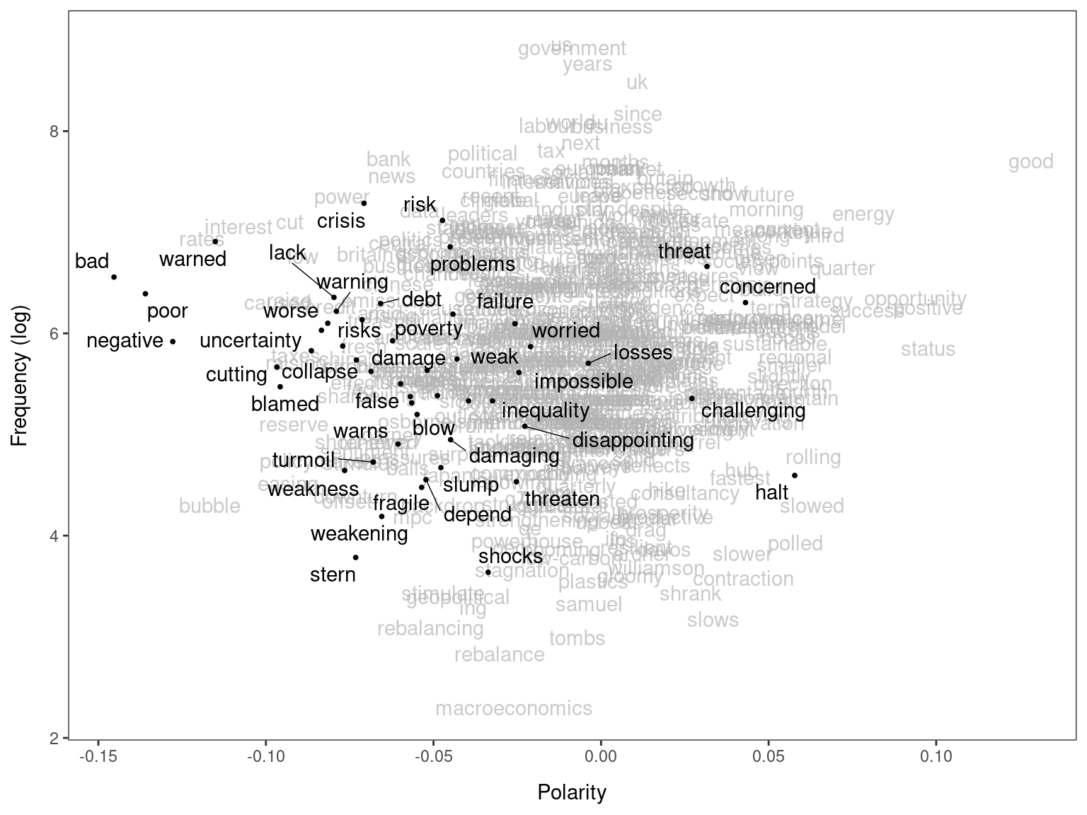
By highlighting negative words in a manually compiled sentiment dictionary (data_dictionary_LSD2015), we can confirm that many of the words (but not all of them) have negative meanings in the corpus.
textplot_terms(tmod_lss, data_dictionary_LSD2015["negative"])
## Warning: ggrepel: 8 unlabeled data points (too many overlaps). Consider
## increasing max.overlaps
We must reconstruct original articles from their sentences using dfm_group() before predicting polarity of documents.
dfmat_doc <- dfm_group(dfmat_sent)
dat <- docvars(dfmat_doc)
dat$fit <- predict(tmod_lss, newdata = dfmat_doc)
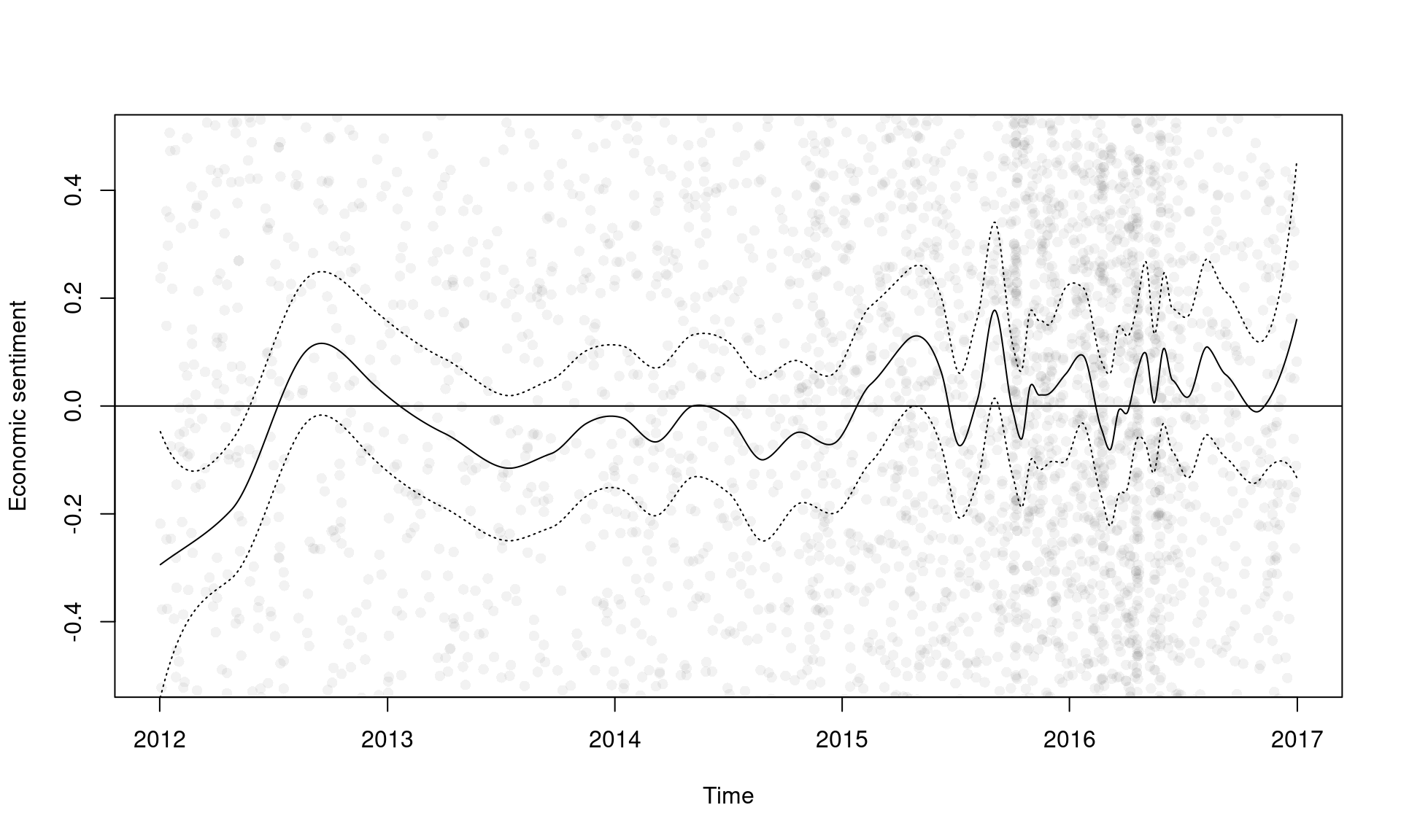
We can smooth polarity scores of documents to visualize the trend using smooth_lss(). If engine = "locfit", smoothing is very fast even when there are many documents.
dat_smooth <- smooth_lss(dat, engine = "locfit")
head(dat_smooth)
##         date time        fit    se.fit
## 1 2012-01-02    0 -0.2941611 0.1258069
## 2 2012-01-03    1 -0.2933006 0.1238591
## 3 2012-01-04    2 -0.2924451 0.1219494
## 4 2012-01-05    3 -0.2915943 0.1200775
## 5 2012-01-06    4 -0.2907481 0.1182429
## 6 2012-01-07    5 -0.2899064 0.1164455
In the plot below, the circles are polarity scores of documents and the curve is their local means with 95% confidence intervals.
plot(dat$date, dat$fit, col = rgb(0, 0, 0, 0.05), pch = 16, ylim = c(-0.5, 0.5),
     xlab = "Time", ylab = "Economic sentiment")
lines(dat_smooth$date, dat_smooth$fit, type = "l")
lines(dat_smooth$date, dat_smooth$fit + dat_smooth$se.fit * 1.96, type = "l", lty = 3)
lines(dat_smooth$date, dat_smooth$fit - dat_smooth$se.fit * 1.96, type = "l", lty = 3)
abline(h = 0, lty = c(1, 2))
- Watanabe, K. 2021. “Latent Semantic Scaling: A Semisupervised Text Analysis Technique for New Domains and Languages". Communication Methods and Measures 15(2): 81-102.
- Watanabe. K. 2023. “Introduction to LSX: The package for Latent Semantic Scaling".