Simple frequency analysis
require(quanteda)
require(quanteda.textstats)
require(quanteda.textplots)
require(quanteda.corpora)
require(ggplot2)
Unlike topfeatures(), textstat_frequency() shows both term and document frequencies. You can also use the function to find the most frequent features within groups.
Using the download() function from quanteda.corpora, you can retrieve a text corpus of tweets.
corp_tweets <- download(url = "https://www.dropbox.com/s/846skn1i5elbnd2/data_corpus_sampletweets.rds?dl=1")
We can analyse the most frequent hashtags by applying tokens_keep(pattern = "#*") before creating a DFM.
toks_tweets <- tokens(corp_tweets, remove_punct = TRUE) %>%
               tokens_keep(pattern = "#*")
dfmat_tweets <- dfm(toks_tweets)

tstat_freq <- textstat_frequency(dfmat_tweets, n = 5, groups = lang)
head(tstat_freq, 20)
##              feature frequency rank docfreq     group
## 1           #twitter         1    1       1    Basque
## 2     #canviemeuropa         1    1       1    Basque
## 3             #prest         1    1       1    Basque
## 4           #psifizo         1    1       1    Basque
## 5     #ekloges2014gr         1    1       1    Basque
## 6            #ep2014         1    1       1 Bulgarian
## 7         #yourvoice         1    1       1 Bulgarian
## 8      #eudebate2014         1    1       1 Bulgarian
## 9            #велико         1    1       1 Bulgarian
## 10 #savedonbaspeople         1    1       1  Croatian
## 11   #vitoriagasteiz         1    1       1  Croatian
## 12           #ep14dk        31    1      31    Danish
## 13            #dkpol        17    2      17    Danish
## 14            #eupol         7    3       7    Danish
## 15        #vindtilep         6    4       6    Danish
## 16    #patentdomstol         4    5       4    Danish
## 17           #ep2014        34    1      34     Dutch
## 18              #vvd        10    2      10     Dutch
## 19               #eu         8    3       6     Dutch
## 20             #pvda         8    3       8     Dutch
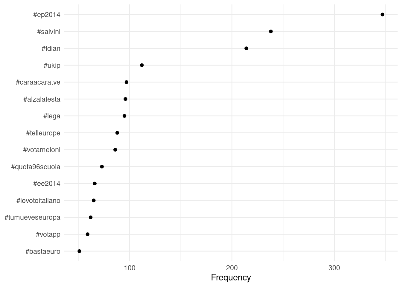
You can also plot the Twitter hashtag frequencies easily using ggplot().
dfmat_tweets %>%
  textstat_frequency(n = 15) %>%
  ggplot(aes(x = reorder(feature, frequency), y = frequency)) +
  geom_point() +
  coord_flip() +
  labs(x = NULL, y = "Frequency") +
  theme_minimal()
Alternatively, you can create a word cloud of the 100 most common hashtags.
set.seed(132)
textplot_wordcloud(dfmat_tweets, max_words = 100)

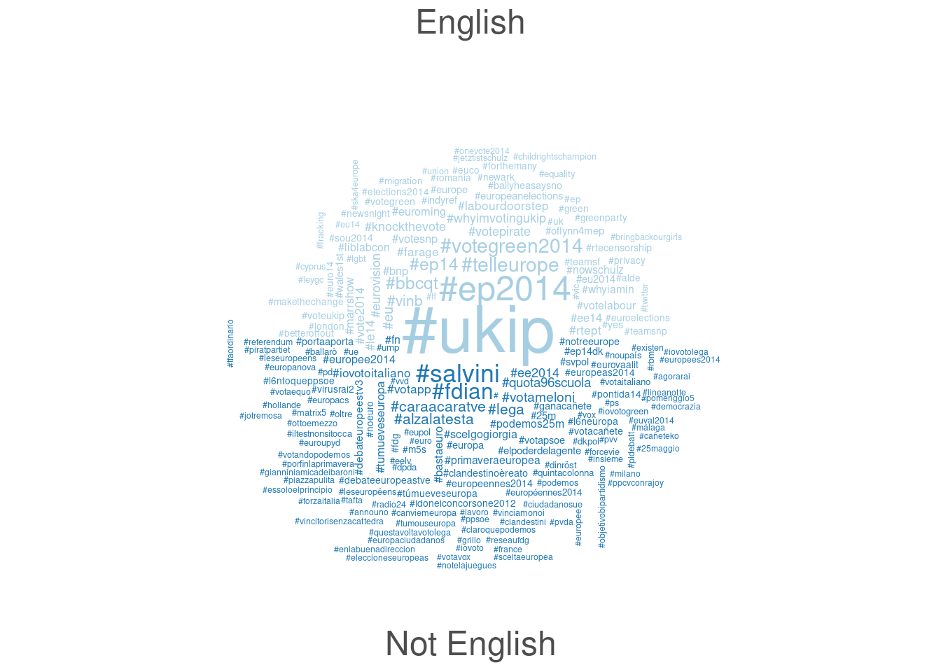
Finally, it is possible to compare different groups within one Wordcloud. We must first create a dummy variable that indicates whether a tweet was posted in English or a different language. Afterwards, we can compare the most frequent hashtags of English and non-English tweets.
# create document-level variable indicating whether tweet was in English or other language
corp_tweets$dummy_english <- factor(ifelse(corp_tweets$lang == "English", "English", "Not English"))

# tokenize texts
toks_tweets <- tokens(corp_tweets)

# create a grouped dfm and compare groups
dfmat_corp_language <- dfm(toks_tweets) %>%
                       dfm_keep(pattern = "#*") %>%
                       dfm_group(groups = dummy_english)

# create wordcloud
set.seed(132) # set seed for reproducibility
textplot_wordcloud(dfmat_corp_language, comparison = TRUE, max_words = 200)